Category: Prediction models

One of the holy grails of COPD research is being able to identify “rapid progressors”, i.e. individuals who are destined for rapid loss of lung function. One of the challenges in doing this in COPD is that the rate of disease progression is usually slow, so that it (probably) takes years of observation to distinguish a “rapid progressor” from a “nonprogressor.”

In the COPDGene Study, our spirometric datapoints come at 5-year follow-up intervals. After the COPDGene 5-year study visit, there was great interest in being able to identify “rapid progressors” who could be studied intensively at the 10-year visit. At first glance, it might seem natural to look for rapid progressors in the set of individuals who had the greatest lung function decline between visit 1 and visit 2; however as I show below this approach can backfire pretty badly, and it’s a nice illustration of both regression to the mean and the practical importance of measurement error. The three COPDGene study visits are shown below. When we built the prediction model we were at the 5-year time point using the visit 1 and 2 data to try and predict behavior at visit 3. Now, we have roughly have of the visit 3 data available to us, so we can learn some things about how successful we were at prognosticating from the five-year visit.

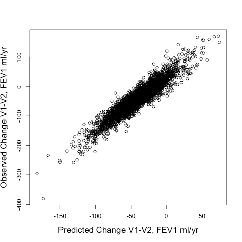
When we tried out different ways to identify rapid progressors, we compared two approaches: 1) Defining rapid progressors based on the observed change in FEV1 from Visit 1 to Visit 2 (observed delta FEV₁^V1-V2) or 2) Defining rapid progressors based on the predicted change in FEV1 (predicted delta FEV₁^V1-V2) using the output of a random forests model using a standard set of clinical and radiographic predictors. The model’s fit to the observed delta FEV₁^V1-V2 was pretty good. The scatterplot is shown below, and the model explained 87% of the variance of the observed delta FEV₁^V1-V2.

The real question though is how well the model predicted future change in lung function, i.e. the FEV₁ change from V2-V3 (observed delta FEV₁^V2-V3). Here is the correlation of the observed delta FEV₁^V2-V3 to predicted delta FEV₁^V2-V3 obtained by using V2 values of the predictor variables entered into the same prediction model as described above. This model explains 10% of the variance of observed delta FEV₁^V2-V3.

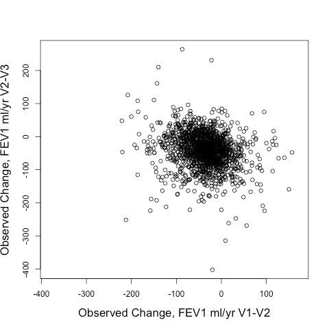
Not great. But interestingly so much better than using the observed delta FEV₁^V1-V2 to predict the observed delta FEV₁^V2-V3. Take a look at the correlation between those two below. It’s negative! In other words, if you want to find rapid V2-V3 progressors, you’d be better off selecting SLOW V1-V2 progressors than you would be selecting rapid V1-V2 progressors.

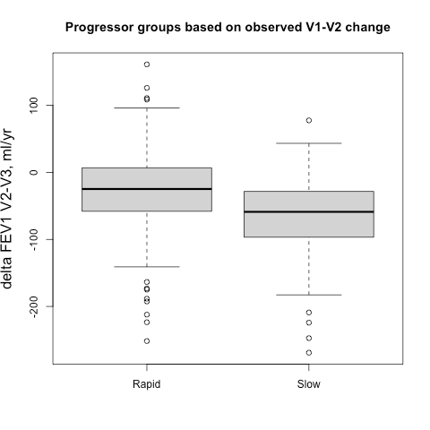
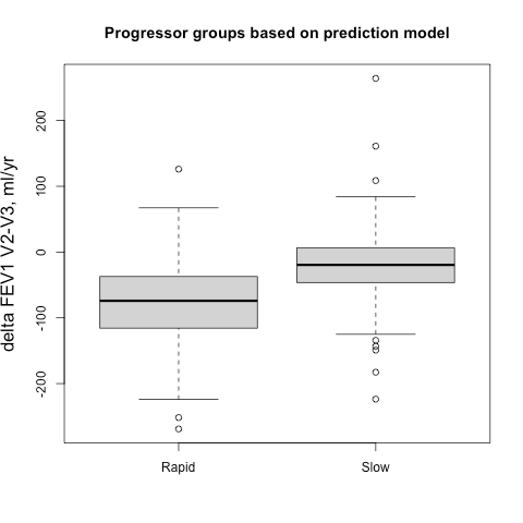
Sometimes it easier to see this when subjects are broken into groups, so we identified groups of 500 fast and slow progressors (stratified by gender to account for differences in lung size) according the their observed delta FEV₁^V1-V2 and their predicted delta FEV₁^V1-V2, and then we compared the prospective 5-year progression of these groups (observed delta FEV₁^V2-V3). These results are shown side-by-side below. It’s apparent that for the groups defined by observed change you actually get the opposite of what you want. The slow group progresses more rapidly over the next five years, but if you rely on the output from the prediction model you get the desired behavior. A t-test comparing the V2-V3 FEV₁ change between rapid and slow groups is highly significant.

• 

• 

This is simple regression to the mean, but can still be counterintuitive. We had to look at the data a bit to really absorb the magnitude of this effect. I think one of the learning points here is that when FEV₁ is observed only twice over relatively short time period, the delta FEV₁ variable can be really noisy. When cutoffs are applied to a variable with low signal to noise ratio, the selected subjects at the extremes of the distribution also happen to be the ones with the largest measurement errors. Those subjects are not actually the ones with the greatest rate of “true progression,” they are just the ones with the largest measurement error that, by virtue of the thresholding, tend to all be aligned in the same direction. Then, if the measurement errors at visit 2 and visit 3 are independent, then the measured FEV₁s of those subjects will move in the opposite direction at the next time point since those measurement errors will be evenly distributed around a mean of zero.

“All science is either physics or stamp collecting.” The implication of this famous quote, attributed to Ernest Rutherford, is that physics, with its mathematical quantification of natural laws, is superior to disciplines like biology that accumulate observations without synthesizing them through mathematical description. From this math-centric perspective, the data revolution in biology is a step up the purity ladder towards physics and away from the social sciences. Despite the odiousness of this reductive view, the biology-physics analogy is enlightening to the extent that it prompts critical thinking about where biology is headed and what the phrase “biology is a data science” might imply. Can the proliferation of new biological data be leveraged to discover the fundamental rules that govern biological systems? Or will we simply end up with billions of stamps and expensive storage bills?

Now that biologists can generate millions of data points from a single sample, it is often assumed that fundamental insights will follow. If one takes the beginning of the Human Genome Project(1990) as the start of the genomics era, we are now 30 years in and still at the stage of large-scale stamp accumulation. The sheer size of a new data set remains one of the major selling points for new papers, and significant time and resources continue to be devoted to the generation of new biological data. Whereas one might have wished for early quantitative breakthroughs from all of this new data, the most obvious short-term effect of genomic technology has been to turn biologists from artisinal into industrial stamp collectors. The fact that the word “landscape” is a staple of high profile genomics papers reflects the degree to which data generation continues to be a primary focus of genomics research.

So, after describing all these landscapes, what comes next? Will genomics be the Bob Ross of science or can we hope that the descriptions of all these landscapes are building towards some kind of quantitative synthesis? Like Einstein in the patent office, is biology’s next quantitative genius is currently designing recommender systems by day and dreaming about fundamental biological principles in her spare time? While it would be great for a new biological synthesis to emerge unexpectedly, most people think that the breakthrough insights in biology will emerge in a more systematic manner through the application of algorithms to big biological datasets. This is where machine learning (ML) comes in.

It is important to avoid a naive faith that ML will magically extract truth from big data. I encounter this ML-centric magical thinking with depressing regularity in biomedicine, and I can personally attest to the many useless ways that ML can be applied to biological data. Too often, the goals of ML-based biology projects are poorly defined, with ML playing a deus ex machina kind of role. These projects don’t adequately account for biological complexity and the limitations of biological data. It’s much easier to use algorithms to identify cats in pictures than to identify the molecular drivers of colon cancer, never mind more detailed questions like why the incidence of early colon cancer is increasing in high income countries. As expert ML practitioners know, domain knowledge is usually an essential ingredient for successful projects.

A compelling roadmap for ML in biology can be found in Yu and Ideker’s “Visible Machine Learning,” which makes use of the Visible V8, a toy engine, as its organizing principle. Just as mechanics need to understand how an engine works in order to repair it, so biologists need to understand how organisms work in order to understand biology and cure diseases. The Visible V8 approximates a true engine closely enough that important lessons about real engines can be learned by studying it. Thus the authors propose that when ML is applied to biological data, the emphasis should be on developing visible (i.e. interpretable) ML models, because the biological insights will come primarily from the structure of the models themselves rather than the model outputs.

This is a great way of thinking about how to use ML with biological data. In this paradigm biology, in its fully-realized quantitative form, will be more like engineering than physics as a discipline. Like engineers, most biologists are interested in learning about how a specific system works. For example, since my research focus is human lung disease, I am relatively (but not entirely) uninterested in understanding lung disease in hamsters or horses. Biologists study contingent systems with specific evolutionary histories, and therefore biology truths are more context-dependent than physics truths. Much of biological research is motivated by understanding how specific organisms solve specific problems within the constraints of physical laws. In biology, context almost always matters, a fact that informs the main arguments of Yu et al. in favor of visible machine learning in biology.

Data Heterogeneity

Yu et al. point to data heterogeneity as a major challenge for applying ML algorithms to biological datasets. In their words, “biological systems are almost certainly more complex than those addressed by machine learning in other areas.” Imagine that you are given a dataset with one million pictures of cats. A standard ML problem might be to identify the cat in each of the pictures. In contrast, a standard biology ML problem would be more akin to getting one thousand fuzzy pictures with noisy labels, and the task is to find out what kind of animals might be in the pictures.

To get more concrete, a fairly well-formulated ML problem is to take a series of gene expression datasets and infer the gene regulatory model that generated these data. Gene expression is partly governed by other genes, and the regulatory connections between genes can be expressed as a network or graph. The problem can then be formulated as one of learning which graph, from the space of all possible graphs, represents the true gene regulatory model that produced the training data. Data heterogeneity complicates this problem in two ways:

• the true model may contain redundancies such that identical output can arise from different inputs
• the data may arise from more than one model, or may be informative for only certain aspects one overall model

With respect to real gene regulatory networks, we know that these networks work differently in different cell types. Some genes, like RFX1, can activate gene expression in one state while inhibiting gene expression under different conditions. The information content of any given biological dataset is often low with respect to the complexity of the generative model, thus, even the biggest biological datasets aren’t really that big relative to the scope of the problem. This is one reason why, 30 years into the genomics era, we are still mapping biological landscapes and we haven’t yet begun to exhaust the space of possible biological states in need of characterization.

Visible, Interpretable Biological Models

So what do Yu et al. mean by “visible” biological models? They don’t give a precise definition, but they state that visual models incorporate “prior knowledge of biological structure.” Interestingly, this presupposes that biological knowledge is encoded and accessible to algorithms, which is its own challenge. But if one assumes that appropriate encodings are available, visible algorithms are a tool for synthesizing prior biological knowledge and novel data. The defining feature of visible models is that their “internal states” can be accessed for further study. Here, visible essentially means interpretable, and the authors make the strong claim that interpretable biological models reflect causal processes in biological systems.

But how can we know that an interpretable model faithfully recapitulates causal processes? One big problem with the Visible V8 analogy is that we already know that the model is a faithful representation of the real thing, but with biological models there isn’t a frame of reference based on reliable ground truth. Our prior biological knowledge is not extensive enough to be at all comparable to the Visible V8. Yu et al. propose that algorithms should include prior information on biological structures, but this does not really ensure that the “internal states” of these models recapitulate the underlying biological reality at a meaningful level of detail. In fact, as I’m sure the authors would agree, they surely don’t. There is a chicken and egg problem here – if we really knew the biological models we wouldn’t need to do ML, but the model is so complex that we are hoping that ML + data can help us to discover it. Some might respond that “all models are wrong but some are useful,” but the visible ML argument relies upon interpretation of internal model states as if they were causal factors, so it is of course important that the states have some meaningful connection to the true model.

Rashomon sets

An important problem for the Visible Models framework is that accurate models don’t necessarily have internal states that reflect causal processes. In an excellent opinion piece on interpretable models, Cynthia Rudin points out that equivalent predictive accuracy for the same task is often achieved by several different methods, implying that there is not a single “best” model but rather a set of different but functionally equivalent models. This set of equivalent models is a Rashomon set (a reference to a famous Japanese movie about multiple perspectives on the same event), and Rudin argues that when the Rashomon set is large there is a reasonable chance that it includes an interpretable (but not necessarily causal) model.

Interestingly, Rudin briefly entertains the causal argument – “Why is it that accurate interpretable models could possibly exist in so many different domains? Is it really possible that many aspects of nature have simple truths that are waiting to be discovered by ML?” – but then she opts for a more conservative argument for interpretable models based on Rashomon sets. The fact that the argument for visible models in biology depends on the claim that these models are approximately accurate reflections of nature is problematic. I personally think it is reasonable, but the onus is on the biology ML community to demonstrate that it is possible to generate models in which studying their internal states produces meaningful biological insights. While there are multiple examples of using prior biological knowledge to guide ML, some of which we have adopted in COPD genomics, I would say that the effectiveness of this approach has not yet been conclusively demonstrated.

Encoding (and updating) biological knowledge

Current ML models don’t closely approximate biological systems, except in very specialized experimental situations. Humans, the systems that we care most about, are incredibly complex multi-cellular, multi-tissue systems with long life spans such that even the most intensive genomic data collection would only capture a small fraction of our biological states. Large-scale landscape projects like the ENCODE, Roadmap Epigenomics, and FANTOM projects have generated tens of thousands of datasets using hundreds of assays to capture biological states in human and murine cell types, and we still know relatively little about how these landscapes change in specific disease or cell activation states. And we haven’t really begun to examine the connectivity patterns between cell types in tissues from a genomic perspective. The bottom line is that, in the short and medium term, we will be in a data poor situation with respect to the complexity of the true biological model. Accordingly, the visible model approach leans heavily on the incorporation of biological knowledge to constrain the model space, presumably ensuring that the resulting models will be representative of “true biology.”

This solution runs the risk of being trivial if, as is often done, results are validated by referencing back to known biology in standard and potentially circular ways. If we are going to use biological knowledge as a constraint, we should focus on examining the internal model states that are initialized by prior knowledge before and after training to determine how they have changed, and we need ways to determine whether these changes are good or bad. Yu et al. propose experimental validation as a means to verify biological predictions arising from the examination of internal model states, which is reasonable but resource intensive. Another alternative is to demonstrate that biologically constrained models objectively improve prediction accuracy relative to unconstrained models. Before you object and state that unconstrained models will always outperform constrained or interpretable ones, consider Rudin’s warning against precisely this assumption. To quote her directly, “There is a widespread belief that more complex models are more accurate, meaning that a complicated black box is necessary for top predictive performance. However, this is often not true, particularly when the data are structured, with a good representation in terms of naturally meaningful features.” After all, the ideal amount of complexity for a model is the amount required to capture the true model, additional complexity just invites overfitting.

I agree with Rudin, because we have shown this to be true in our own domain. By incorporating information related to gene splicing into a previously published gene expression predictive model for smoking behavior, we significantly improved prediction accuracy in test data.

The best performing models were deep neural nets that included an isoform-mapping-layer (IML) manually encoded to represent known relationships between exons and transcript isoforms. Interestingly, we know that this information is only partially accurate, but it still provides enough information to clearly boost accuracy. With additional modifications, it should be possible to update the IML with strong patterns of correlated expression between exons that indicate as yet unidentified transcript isoforms. In this scenario, ML is part of a virtuous cycle in which prior biological knowledge in coded structures guides ML discovery, and ML discovery updates these structures. These structures then become continuously evolving repositories of biological knowledge. I would argue that it is this cycle and these structures that are the desired endpoint of biology as a data science – not static formulas like E = mc², but a continuously evolving encyclopedia of algorithms and data structures.

Final thoughts

So, how should we go from describing genomic landscapes to understanding the rules that shape these landscapes? I agree with Yu et al. in their overall endorsement of interpretable algorithms that integrate prior knowledge with new data. At present the methods to interrogate internal states are vague, and further development in that area is needed. As Rudin states, interpretability is domain specific, and while Yu et al. have begun to define what interpretability means in the biological domain, this needs to be defined more precisely so that standardized comparisons between algorithms can be more readily made. Finally, the biggest challenge is to prove that the internal states of ML models mean anything at all. For many biological problems, the size of the Roshomon set is large. The use of prior biological knowledge to constrain ML models is a natural solution to this problem, but this establishes a new problem of encoding a wealth of biological facts into data structures that can interact with new data via algorithms. Biologists should and will continue to characterize biological landscapes, but we also need an expandable canvas of algorithms and data structures that can link these disparate landscapes into interpretable models of biological systems.