Tree-based models (random forests, XGBoost) are usually among the top performing methods for tabular datasets, so there is substantial interest in this method that claims to compute fast, exact SHAP scores for tree-based models. In reviewing this within our group we spent a lot of time figuring out some specific aspects of proper calculation and interpretion of SHAP scores which will be recorded here for future reference. As shorthand, this method for calculating SHAP scores will be referred to now as the tree explainer.
This post is based on the following papers/sources:
- The Lundberg 2017 original SHAP paper (“A Unified Approach to Interpreting Model Predictions”)
- The Janzing 2020 AISTATS paper pointing out a conceptual issue with the original SHAP paper (“Feature relevance quantification in explainable AI: A causal problem”)
- The Lundberg 2020 paper describing the Tree SHAP method (“From local explanations to global understanding with explainable AI for trees”)
- The Tree SHAP implementation docs
First, how does the tree explainer actually work? First, there are multiple implementations of the explainer, but I think that the “path dependent” implementation is the easiest to understand. This is the algorithm description from a preprint of the paper.
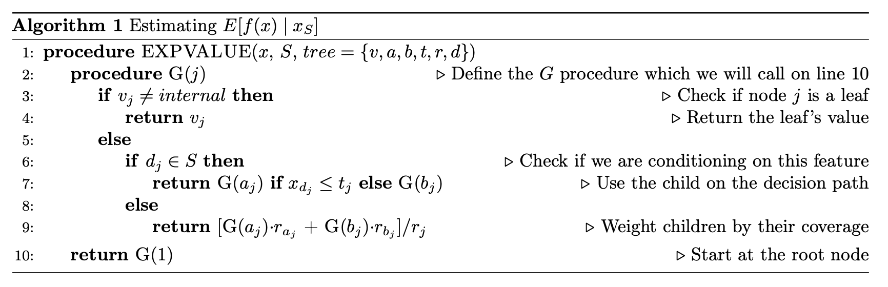
To understand what v,a,b,t,r, and d are, this part helps.
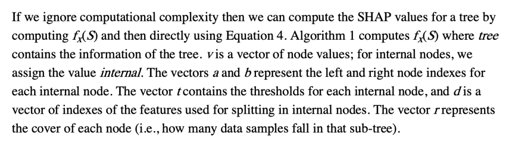
Some important points to make about this:
- This does not require any data, and can be computed directly from the trees
- It does however require the coverage of each node in order to compute a weighted average. In many tree-based models, this is stored along with the trees and correspond to how many training examples “went through” a given node.
- “Conditioning on” must be understood properly, and there is a later section dedicated to this
- Line 9 means that when a feature is being conditioned on, which is the same as being dropped or excluded (if you don’t understand this aspect of calculating SHAP scores, you basically just need to go back to the basics of what SHAPs are and how they are calculated), the way this is implemented in the trees means that “dropping a feature” in effect means replacing that feature with its average, which more specifically translates to the average of its effects in the training dataset.
- This will then give us a vector of model predictions where the feature of interest is dropped. The vector is of length equal to the number of observations of the feature, and the the SHAP value for each observation will be the difference between the prediction from the full model and the value output by this algorithm for that observation. The resulting vector consists of what we often call “local SHAPs” (observation-specific importance of a feature) and the sum of this vector is the “global SHAP.” (total importance of a feature over all observations of interest)
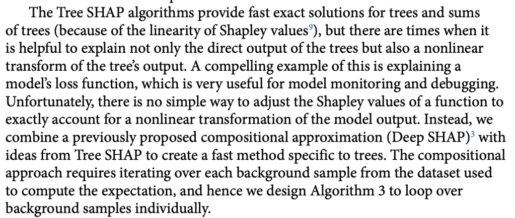
If you’re following along with the original paper, we skip discussion of the next algorithm (Algorithm 2 in the paper), which the authors claim to simply be a more computationally efficient (but empirically equivalent) implementation of the algorithm we just reviewed.
Things get interesting (in a scientific method, gossipy kind of way) with Algorithm 3 (Tree SHAP with interventional perturbation). For reasons I don’t fully understand (TBH), the interventional perturbation algorithm is necessary if one wants to calculate SHAP values not for the model’s direct output, but for a nonlinear transformation of the model’s output. It seems like Algorithm 3 does what Algorithm 2 does, but it does this by iteratively looping over individual observations (which means real data, not just the trees, is required). This is described here.
The gossipy interesting part is this. In the original SHAP publication, the authors theorized that the best way to compute SHAPs would require having access to the conditional expectation of the model prediction. What is this? It is the average prediction that the model would make if the variable of interest (the one being conditioned on) was not available to the model. One way of thinking about this which is not exactly correct I think is that, in order to calculate this, we need to know what the prediction of the model would be for each observation if one feature was removed and the rest of the feature values were the same as they actually were for that observation. Since it is hard to compute the conditional expectation, the authors in the original paper basically did the right thing for the wrong reason – namely the used the marginal expectation instead claiming that would be OK if one assumed that all features were independent. In this subsequent paper, a different set of authors explains that the marginal expectation was actually the right thing to use all along, and that people had been and were still at risk of making future errors by trying to “improve” SHAP methods by using the conditional expectation. The relevant portions are included below.
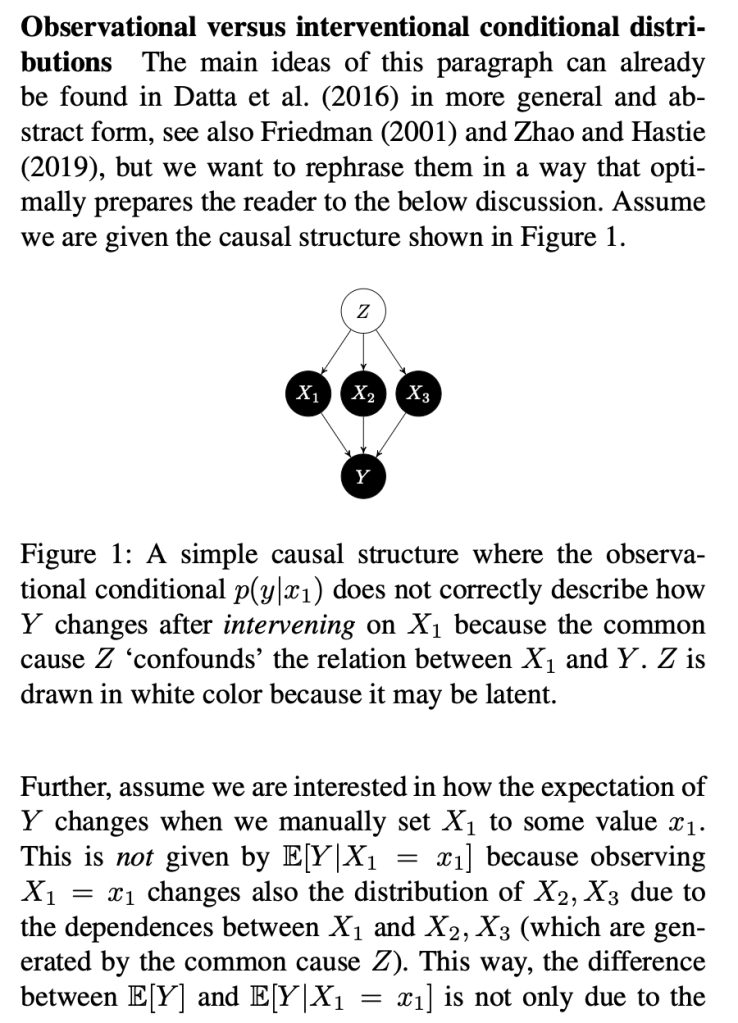
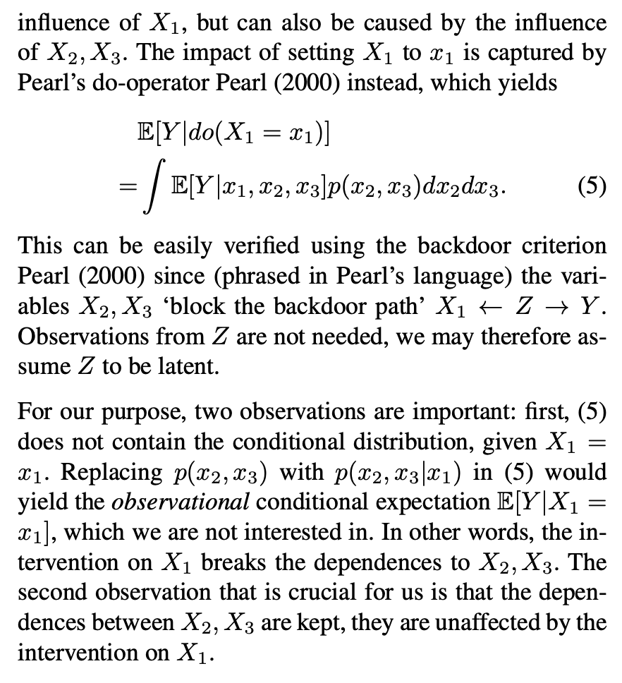
The key thing here is the reference to causal theory and the do-operator. The practical point is that by using the do-operator, we can calculate the expected prediction for a specific value of a variable (a specific value of x1 for a variable X1 that we wish to get a SHAP value for), accounting for the full joint probability distribution of x2 and x3 (or the rest of the features, however many there are). I think the reason why this is called an interventional conditional distribution is that do-operator allows for us to intervene on X1 by enforcing a specific value in a manner that is robust to spurious attributions of importance that can arise from correlation patterns in observational data that can arise from unobserved variables. Some important points that follow from this:
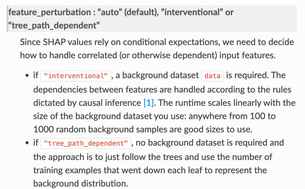
- In the shap.TreeExplainer implementation, when feature_perturbation is set to “interventional”, this is what is being done and the reason why real data are needed is in order to get a reasonably accurate estimate of p(x2,x3), i.e. the multivariate distribution of all of the variables (except for X1).
Some other open questions.
- So what data should we provide when we are using the tree explainer?
- Some relevant info: It seems that the “expected_value” used in the tree explainer comes from the model itself, not from any specific provided data. This depends on the model object including the coverage for each node, and this means that the expected_value is equivalent to the mean of the predicted values in the training dataset (accounting for in some methods some random variation from random sampling in the training procedure, as discussed here).
- Assuming the thing above, then the main concern for what sort of data to provide relates to the “interventional” behavior described above, which means that it is probably not every really necessary to provide the entire training dataset to the tree explainer.
- end